The stability of peri-urban croplands globally:

An approach to examine exposure to climate extremes

Author

Affiliation

Published

2024-05-01

Abstract

Croplands are subject to a variety of pressures, including the influence of urban expansion on cropland area and the impacts of climate change on crop yield. As the world’s population becomes increasingly urbanized, there is a growing need to understand the relationship between urban areas and the surrounding ‘peri-urban’ croplands in their hinterlands. However, global-scale analyses face a challenge of inconsistencies in the boundaries to assess peri-urban croplands and thus local food production. My thesis addresses this gap by applying a consistent travel-time-based approach and a high-resolution global cropland map to delineate the peri-urban cropland catchment of 2,425 urban centres with populations greater than 250,000 worldwide. I then calculated the stability of cropland over a 16-year period between 2000 to 2019 within these catchments, which revealed sharp geographic differences among urban centres in terms of their peri-urban cropland change dynamics. Applying these catchment boundaries, I then present a procedure that can be used to determine crop-specific exposure to extreme heat in these peri-urban croplands. Current studies of cropland’s exposure to extreme temperatures tend to focus on regional and continental trends, with less emphasis on local agriculture specific to individual cities. Specifically, I describe a subset of urban areas (n=929) with a minimum cropland area of 10% within their catchments alongside a condition that 80% of that cropland was stable between 2000–2003 and 2016–2019. My proposed approach provides a heuristic that can be applied for specific urban areas globally to help guide land-use planning and climate-adaptation measures to support peri-urban crop production. To identify gaps in the global food system with global urbanization, we need to improve our understanding of where peri-urban croplands are located, how they are changing, and how climate change may impact them.

Introduction

In a rapidly evolving world, we must constantly seek to improve our understanding of how human activity is changing the land—particularly in the case of agriculture and the food system. The world’s populations continue to urbanize, with two-thirds of all people expected to live in a city by 2050 (United Nations 2019). This growth and the associated increase in urban land area has often and will likely come at the expense of the ‘peri-urban’ croplands located on the outskirts of cities (Li, Verburg, and van Vliet 2022; Shaw, Vliet, and Verburg 2020). Alongside changes in cropland area that could affect food production, there is a compounding effect due to climate change, such as the increase in mean temperatures and exposure to extremes that can impact crop yields (Karger et al. 2023). These global changes in temperatures have already begun to have a meaningful impact on the production of key crops by pushing them beyond their physiological limits, which is expected to further increase this century (Ray et al. 2015, 2019; Lobell, Schlenker, and Costa-Roberts 2011; Jägermeyr, Müller, Ruane, et al. 2021). Taken in sum, the loss of peri-urban land used for agriculture and the impacts of climate change on crop yield represents a significant threat to the global food system and a need to understand where and how these shifts will occur.

Considering croplands from an urban perspective

Much of the world’s croplands are located near urban areas, with 60% of all irrigated cropland and 35% of rain-fed cropland within 20 km of a city in 2000 (Thebo, Drechsel, and Lambin 2014). While local agriculture is not typically sufficient to support the full dietary demand of a city, nearby agriculture serves as a meaningful source of key food staples (Kinnunen et al. 2020; Schreiber et al. 2021). However, croplands located around cities can face significant pressures due to urban expansion. In addition to a growing global urban population, built-up land area has been expanding rapidly to support this growth in some regions (Li, Verburg, and van Vliet 2022). This poses a potential threat to peri-urban croplands, which have often been converted to support urban expansion (Shaw, Vliet, and Verburg 2020; Potapov et al. 2022). With their high yields and geographic proximity, the loss of these croplands could undermine the resilience of urban food systems (Nelson et al. 2021; Béné et al. 2016; Seekell et al. 2017). While serving as consumers of nearby agriculture, urban areas directly influence their peri-urban regions through their policy decisions and their contributions to higher temperatures (Shaw, Vliet, and Verburg 2020; Tuholske et al. 2021). Considering the deep interconnections that cities have with their hinterlands, municipal policies and planning must be central in any discussion of local agriculture; they serve as a key determinant of the success of peri-urban food production (Schreiber et al. 2023).

The foodshed and its relevance to urban centres

When discussing a city’s local food system, the simplest approach is to consider its ‘foodshed’. A foodshed is the agricultural catchment of a population centre that can exist at the local, regional, and global scales (Kinnunen et al. 2020). The concept of a foodshed has tended to follow one of two definitions in the literature, as described by Schreiber et al. (2021), with some studies identifying a foodshed as “the actual geographic areas from which a population sources its food” while others treat a foodshed as “any area with the potential to feed a given population” (Original discussion by Peters et al. 2009). This is a crucial distinction: studies attempting to model foodsheds require abstractions based on the production capacity and consumption of an area, which can entail considering agricultural trade and complex food flows (Karg et al. 2023). At the global scale, this can be seen in Kinnunen et al. (2020), who define a foodshed as “areas linked together through movement and consumption of food,” though their study relies on modelled agricultural trade flows and thus falls into Schreiber et al.’s (2021) definition of the potential food sourcing regions. The application of a foodshed also can be seen in studies that do not use the term. For example, Nelson et al.’s (2021) assessment of the resilience of international and domestic agricultural trade networks echoes the foodshed concept through its focus on the inherent spatial links within and between nations. Modelling these inter- and intra-national agricultural networks to determine global foodsheds is a complex and resource-intensive task, with current leading efforts requiring complicated methodologies and assumptions while remaining fairly coarse-grained (Kinnunen et al. 2020; Nelson et al. 2021).

Due to the difficulty of determining the real-world foodshed of a city and the complexity of undertaking a global approach to foodsheds, I chose to focus on examining croplands at the peri-urban scale, which could be thought of as part of an idealized local foodshed (Peters et al. 2009). While my hypothesis is that local peri-urban crop production is likely insufficient to support the demands of most urban areas for some crops (such as grains and a wide array of fruits), it could play a more pivotal role in providing certain crops, such as pulses, roots, and other vegetables¹. Considering the myriad impacts that cities can have on their peri-urban regions, it is pivotal to address each urban area individually to facilitate each area’s actions to benefit nearby agriculture.

Examining the impacts of climate change on local crop production

It is well established that global temperatures have been rising and will continue to do so, which will have a host of impacts on agriculture globally (Heino et al. 2023; Jackson et al. 2021; Zhu and Troy 2018; Jägermeyr, Müller, Ruane, et al. 2021). However, there are important nuances to consider. An area’s terrain can have a notable impact on its climate and can moderate increases in temperature (Karger et al. 2023). While studies have investigated the exposure of urban areas to temperature extremes and others have examined rural agriculture’s exposure to extreme temperatures, no studies have tackled both (Mueller et al. 2016; Tuholske et al. 2021). We could therefore expect that peri-urban croplands would be subject to a unique climatic exposure. This, to my knowledge, has not been fully studied (especially at the global scale).

Several methods have been used to determine cropland’s exposure to extreme temperatures. Due to variation in their distribution and physiology, different crops can have vastly different tolerance for extreme temperatures that continue to evolve with changing temperatures (Butler and Huybers 2013; Jackson et al. 2021; Song et al. 2022). In particular, when crops are exposed to extreme temperatures during their growing period, they degrade rapidly in a non-linear trend (Schlenker and Roberts 2009; Butler and Huybers 2013). This results in a conundrum for croplands near cities, as they are subject to similar heat exposures as urban areas, but have a greater proportion of evapotranspirative cooling (Findell et al. 2017). Many studies tackle this by establishing a threshold temperature, above which a crop’s yield begins to suffer. In practice, this means identifying any daily maximum temperature that exceeds a threshold as a Killing Degree Day, or KDD (Jackson et al. 2021; Zhu and Troy 2018). However, this requires establishing a threshold for every crop considered, which is difficult and uncertain (Song et al. 2023; Butler and Huybers 2013). For example, in their analysis of cropland intensification and centennial trends in the summer climate of the U.S. Midwest, Mueller et al. (2016) identified the 95th percentile of daily maximum summer temperatures (June-August) that crops are exposed to; however, while relatively simple and consistent, this is an innately comparative approach.

Objectives and research questions

In this thesis, my primary goal was to evaluate the exposure of peri-urban croplands to extreme temperatures. However, this required a first step to assess city-specific peri-urban cropland areas (local foodsheds) and their stability over time, leading me to the travel-time-based approach to determining the influence of an urban area pioneered by Cattaneo, Nelson, and McMenomy (2021). Because their study focused on the ‘urban-rural continuum’ more generally (a classification irrespective of any single city), rather than the catchments of individual cities, this led me to generate my own peri-urban foodshed catchments for 2,425 individual urban centres. Additionally, due to the pioneering work of Weiss et al. (2020), these catchments were modern (representative of 2019), but it is unreasonable to assume that these catchments (and the croplands within them) have remained in the same location and extents for the full duration of a climate-centred analysis. To address this concern, I calculated the stability of cropland within these peri-urban foodsheds, which offers a novel perspective into the changing food systems in many regions. While my primary focus on assessing the extreme temperature exposures was stymied by processing limitations, I propose a heuristic to complete such an anlaysis in the future.

Methods

My thesis proceeded in three major steps: the generation of the travel-time based foodsheds, assessing the stability of cropland within these foodsheds, and comparing each foodshed’s exposure to extreme heat. The foodsheds were generated at the 60-, 180-, and 300-minute ranges for each individual urban centre present in the Global Human Settlement Layer Degrees of Urbanization dataset (Schiavina, Melchiorri, and Pesaresi 2023). Then, using temporal cropland data for 2000–2003 and 2016–2019, I calculated the total cropland within each foodshed and the amount of stable cropland². To ensure that agriculture within the foodsheds were stable for the extent of the extreme temperature analysis, a filter for a total cropland amount of \(\ge10\%\) and a stable cropland amount of \(\ge 80\%\) was applied. I then establish an approach for determining the crop-specific exposure to extreme heat for each selected foodshed.

Input Data

Table 1: Input data sources with their respective uses, temporal information, resolution, and coordinate reference system.
Name	Method	Time Period	Spatial Scale	CRS	Usage	Source
GHS-SMOD	Foodshed generation	2020	1 km	World Mollweide, EPSG:54009	Urban centre identification	Schiavina, Melchiorri, and Pesaresi (2023)
GHS-POP	Foodshed generation	2020	1 km	World Mollweide, EPSG:54009	Population filtering	Schiavina et al. (2023)
GHS-UCDB	Foodshed generation	2015	1 km³	WGS 84 (EPSG:4326)	Population filtering and settlement names	Florczyk et al. (2019)
Global Motorized Friction Surface	Foodshed generation	2019	30 arc seconds (~0.92 km @ equator)	WGS 84 (EPSG:4326)	Accessibility surface generation	Weiss et al. (2020)
Potapov Cropland	Cropland stability	2000–2003 and 2016–2019	0.9 arc seconds (~30 m @ equator)	WGS 84 (EPSG:4326)	Crop-agnostic cropland area	Potapov et al. (2022)
MIRCA2000	Crop-specific extreme temperature exposure	2000	5 arc minutes (~9.2 km @ equator)	WGS 84 (EPSG:4326)	Crop-specific and irrigation method-specific harvested areas	Portmann, Siebert, and Döll (2010)
GGCMI Phase 3 crop calendar	Crop-specific extreme temperature exposure	?	30 arc minutes (~55.6 km @ equator)	WGS 84 (EPSG:4326)	Crop-specific and irrigation method-specific crop calendars	Jägermeyr, Müller, Minoli, et al. (2021)
CHELSA-W5E5	Crop-specific extreme temperature exposure	1986–2016⁴	30 arc seconds (~0.92 km @ equator)	WGS 84 (EPSG:4326)	Global daily max temperature values	Karger et al. (2023)

Travel-time-based foodshed generation

Determining the boundary of an urban centre

flowchart TD

A[("GHS-SMOD (2020)")] --> B(Select all urban centres)

B --> C(Convert raster to polygon)

C --> D(Remove non-urban centre polygons)

D & F[("GHS-POP (2020)")] --> E(Sum the population contained within the urban centres)

G[("GHS-UCDB (2015)")] --> H(Project to 1 km Mollweide)

H & E --> I("Spatially join the urban centres of GHS-UCDB (2015) to
            the generated urban centres with the greatest overlap")

I --> J[Export urban centre polygons] & K(Generate points every 500m<br/>along the edge of each urban centre)

K --> L(Project points to WGS 1984)

L --> M[Export urban centre boundary points]

Figure 1: Workflow for generating the urban centre polygons and points that were used in Figure 2. This procedure was adapted from the work of Cattaneo, Nelson, and McMenomy (2021).

Due to its open-access, high-quality, and frequent use in the literature, I make use of the European Commission’s Global Human Settlement Layer (GHSL) (Tuholske et al. 2021; Weiss et al. 2018; Nelson et al. 2019; Cattaneo, Nelson, and McMenomy 2021). This takes the form of the GHS-POP (population) layer for 2020, GHS-SMOD (Modeled Degree of Urbanization) layer for 2020, and GHS-UCDB (Urban Centre Database) layer for 2015 (Schiavina et al. 2023; Schiavina, Melchiorri, and Pesaresi 2023; Florczyk et al. 2019).

Using GHS-SMOD, -POP, and -UCDB, I identified each unique urban centre through an adaptation of the methodology established by Cattaneo, Nelson, and McMenomy (2021) (see Figure 1). The urban centres were identified in GHS-SMOD and associated with the population values in GHS-POP and GHS-UCDB, alongside the city and country names provided in GHS-UCDB. Points were then generated every 500m along the edge of the boundaries. As these steps were conducted at 1 km resolution and aligned to the same grid, the final step was to project the data into the same coordinate reference system as the friction surface used to generate the travel-time foodsheds (WGS 84, EPSG:4326).

Once both the urban centre polygons and points were generated, they were imported into R for further processing. There, I separated each urban centre’s points to facilitate later processing. Though a population filter was initially considered, the base filter from GHSL-SMOD’s urban centre classification of \(\ge250\,000\) was maintained.

Post-processing R code for extracting the individual urban centres.

renv::restore() # Use `renv::` to emulate the exact packages used in this paper (some methods now depreciated)
library(rgdal)
library(tidyverse)

# Filtering step, run even if not filtering by population ======================

targetpolygons.filename <- "EXAMPLE/urban_centers_polygon.shp"

targetpolygons <- readOGR(targetpolygons.filename)

ids <- targetpolygons$ID
# This variable is used to identify all individual foodsheds.

GHS_POP_R2023A_2020 <- targetpolygons$GHS-POP_2020

GHS_UCDB_POP_2015 <- targetpolygons$GHS-UCDB_POP_2015

filter_pop <- F # Change to `T` if filtering by population

filter_value <- 1000000 # Adjust to your population value, if using

if(filter_pop == T){
  selected_targets <- tibble(ids, GHS_POP_R2023A_2020, GHS_UCDB_POP_2015) %>%
  # arrange(population) %>% # Include if desired to look at the sorted data frame
  filter(GHS_POP_R2023A_2020 >= filter_value | GHS_UCDB_POP_2015 >= filter_value) %>%
  # Using both GHS-POP_2020 and GHS-UCDB_POP_2015 ensures that any orphaned cells will still be included in processing
  pull(ids)
  
} else {
  
selected_targets <- ids

}

write_csv(selected_targets, "selected_targets.csv")

# Cleaning up
rm(targetpolygons, targetpolygons.filename, GHS_POP_R2023A_2020, GHS_UCDB_POP_2015, filter_pop, filter_value, ids)

# Should end this step with `selected_targets` still in your environment

# Exporting individual boundaries ==============================================

alltargets.filename <- "EXAMPLE/urban_centers_point_wgs1984.shp"

alltargets <- as.data.frame(readOGR(alltargets.filename))

for(target in 1:length(selected_targets)){
print(target) # Tells you what cycle it's on

temp <- alltargets %>%
  filter(ID == selected_targets[target])

export.file <- paste0("EXAMPLE/Boundary/boundary_", selected_targets[target], ".shp") # Edit to your preferred export location
export.layer <- paste0("ID_",selected_targets[target]) # Edit to your preferred layer name

export <- SpatialPointsDataFrame(select(temp, coords.x1, coords.x2), select(temp, !c(coords.x1, coords.x2)))

try(writeOGR(export, export.file, export.layer, driver="ESRI Shapefile"))
print(.Last.value) # Should ping if unsuccessful export

# Clean up
rm(temp, export.file, export.layer, export) 
gc()
}

# Clean up
rm(alltargets, alltargets.filename, target) 
gc()

Generating travel-time catchments for each urban centre

flowchart TD
  C[("Weiss et al. (2020)<br/>Friction Surface")] --> D
  A[Urban centre boundary points] --> B(Separating individual urban centres)
  B --> D(Calculation of urban centre<br/>specific access surfaces)
  E["Cattaneo, Nelson, and<br/>McMenomy (2021) Methodology"] --> D
  D --> F(Trimming extents to 300 minutes)
  F --> G(Merging disjoint foodsheds)
  G --> I(Trimming to finer extents)
  I --> K(180 min)
  I --> M(60 min)
  subgraph "Outputs#nbsp;"
  H[Maximum extent foodsheds]
  L[Regional foodsheds]
  N[Peri-urban foodsheds]
  end
  G --> H
  K --> L
  M --> N

Figure 2: Workflow for generating the travel-time-based foodsheds.

After the separation step, the travel-time catchments were generated for each urban centre (Figure 2). These catchments are typically referred to as ‘accessibility’ surfaces, reflecting the time required to ‘access’ a location and constructed using a ‘friction’ surface which similarly reflects the cost (or ‘friction’) to move through the cell (Weiss et al. 2018). Using Weiss et al.’s (2020) Global Motorized Friction Surface’s high resolution, modern, and global extent, it was possible to generate an accurate and location-specific representation of each urban centre’s peri-urban foodshed. Drawing from the methodology established by Nelson et al. (2019) and Cattaneo, Nelson, and McMenomy (2021) and van Etten’s (2017) implementation of least-cost distance calculations for R, it was feasible to implement this approach in contrast to other methods used (such as distance-based fixed buffers).

R code showing the generation of the travel-time foodsheds.

library(raster)
library(gdistance)
library(rgdal)
library(tidyverse)

# Bring the selected targets back
selected_targets <- read_csv("selected_targets.csv")

# Friction surface selection
friction.filename <- "202001_Global_Motorized_Friction_Surface_2019.tif" # If also using @Weiss2020's friction surface.
friction <- raster(friction.filename)

for (cities in (1:length(selected_targets))){
  print(cities) # Displays what loop through it's on, for debugging

  # Import the city boundary
  targets.filename <- paste0("EXAMPLE/Boundary/boundary_", selected_targets[cities], ".shp")
    # Plural as it selects multiple points, all with the same ID value
  print(targets.filename)
  targets <- readOGR(targets.filename)

# Making the transition matrix for processing
  T.GC.crop.filename <- paste0("EXAMPLE/transition/transition_", selected_targets[cities],".T.GC.rds")
  print(T.GC.crop.filename)

  # A unique transition matrix for each target
  if (file.exists(T.GC.crop.filename)) {
    # Read in the transition matrix object if it has been pre-computed

    T.GC.crop <- readRDS(T.GC.crop.filename)
    print("read in transition matrix")

  } else {
  # Cropping the extent of the friction raster to the selected area
    print("creating the cropped friction surface")
    ext <- extent(targets)

    crop <- ext + c(-5.5, 5.5, -5.5, 5.5)
    # Presumes the target data is in degrees, provides a lot of space, can tune
      # 5.5° x 5.5° appears to be adequate for all latitudes to generate a 5hr (300 min) accessibility surface

    friction.cropped <- crop(friction, crop)
    # Actually crops the friction matrix

    rm(ext)
    rm(crop) # Yeah it's like 16B what about it

  # Make and geocorrect the transition matrix (i.e., the graph)
    print("creating transition matrix")
    T.crop <- transition(friction.cropped, function(x) 1/mean(x), 8) # RAM intensive, can be very slow for large areas
    rm(friction.cropped) # Memory clearing
    T.GC.crop <- geoCorrection(T.crop)
    rm(T.crop) # Memory clearing
    saveRDS(T.GC.crop, T.GC.crop.filename)
    print("transition matrix corrected and saved to file")
  }
  gc()

  # accumulated cost calculation to the nearest target using the geo-corrected graph and the target points. - THIS IS THE ACCESS SURFACE

  print("compute travel time")
  output.raster <- try(accCost(T.GC.crop, coordinates(targets))) 
  
  output.filename <- paste0("EXAMPLE/output/output_", selected_targets[cities],".accessibility.tif") # Edit to your prefered output directory

  # Write the resulting raster
  try(raster::writeRaster(output.raster, output.filename, format="GTiff", 
                          #overwrite=TRUE # commented out for re-runs currently, until proven otherwise
                          ))

  print("access raster saved to file") # Using the try() above ensures that the loop will exit if the writeRaster() returns an error message

  rm(T.GC.crop)
  rm(output.raster)
  gc()
}

After initially creating each travel-time surface, it was in its raw 5.5°² extent. Though an arbitrary cutoff point, 300 minutes was selected as the maximum extent of each urban centre’s catchment, with 180- and 60-minute catchments created to be more representative of their regional and peri-urban foodsheds, respectively. Due to ArcGIS Pro’s default behaviour of using four-point contiguity (instead of eight-point contiguity⁵) when generating polygons from rasters, resulting in some urban centres appearing as separate entities. This was addressed by merging the travel-time surfaces for all of the separated pieces of the urban centres.

R code showing how the travel-time surfaces were trimmed to to their 300, 180, and 60 minute extents and how separated surfaces were joined.

# Triming to the 5hr (300 min) limits ====================================

# Still using the `selected_targets` for ids
library(terra)

for(rasters in 1:length(selected_targets)){
  print(rasters) # Say what cycle it's on
  input.access.filename <- paste0("output/all_5.5x5.5_2023-09-27/output_", selected_targets[rasters], ".accessibility.tif")
  output.filename <- paste0("output/trimmed_300min_output/", selected_targets[rasters], "_trimmed_300min.tif")
  
  input.access <- rast(input.access.filename)
  
  (input.access <= 300) %>% # Select all values less than or within 5 hours
  terra::mask(input.access, ., maskvalues=F) %>% # Mask them off
  terra::trim() %>% # And then trim!
  terra::writeRaster(., output.filename) # And write the output
    # Written with LZW compression (lossless)
}
rm(input.access, input.access.filename, output.filename, rasters)
gc()

# Combining cities that were divided into multiple polygons ====================

# Target polygon info
targetpolygons.filename <- "C:/Users/aclaus2/Documents/GIS Work/Honours/Output/try5/urban_centers_polygon_250000.shp"
targetpolygons <- vect(targetpolygons.filename)
targetpolygons.df <- as_tibble(targetpolygons)

multi_poly_targets <- targetpolygons.df %>% # Making a tibble of possible targets
  select(ID, UC_NM_MN, CTR_MN_ISO) %>% 
  group_by(UC_NM_MN, CTR_MN_ISO) %>% 
  summarise(
    count = n()
  ) %>% 
  filter(count != 1 & !is.na(UC_NM_MN) & ! UC_NM_MN == "N/A") %>% 
  select(!count)

possible_overlap <- targetpolygons[targetpolygons$UC_NM_MN %in% multi_poly_targets$UC_NM_MN]
possible_overlap_cities <- unique(possible_overlap$UC_NM_MN)

# cities <- 2 # for debugging
for (cities in 1:length(possible_overlap_cities)) {
  print(cities)
  temp_nearby <- targetpolygons[targetpolygons$UC_NM_MN == possible_overlap_cities[cities]] %>% 
    nearby(., distance = 20000, centroids = F, symmetrical = F)  %>% 
    as_tibble()
  if (cities == 1) {
    nearby <- targetpolygons[targetpolygons$UC_NM_MN == possible_overlap_cities[cities]] %>% 
      as_tibble() %>% 
      mutate(
        order = row_number(),
        nearby = ifelse(order %in% temp_nearby$from, T, F)
      ) %>% 
      filter(nearby == T) %>% 
      select(ID, UC_NM_MN)
  } else {
    temp_join <- targetpolygons[targetpolygons$UC_NM_MN == possible_overlap_cities[cities]] %>% 
      as_tibble() %>% 
      mutate(
        order = row_number(),
        nearby = ifelse(order %in% temp_nearby$from, T, F)
      ) %>% 
      filter(nearby == T) %>% 
      select(ID, UC_NM_MN)
    nearby <- rbind(nearby, temp_join)
  }
}
nearby <- nearby %>% 
  rename(
    cities = UC_NM_MN 
  )
write_csv(nearby, "output/trimmed_300min_output/combined/key.csv") # Write this key down!
# Could also have gone by those that have the same UCDB_POP_2 value. welp,

  ## Combining the rasters of those multipoly cities ====

key <- read_csv("output/trimmed_300min_output/combined/key.csv") # Read in the key if skipping the above steps 
targets <- unique(key$cities)

# target <- 1 # For debugging
for (target in 1:length(targets)) {
  print(target) # what cycle are we on?
  print(targets[target]) # What city?
  to_mosaic <- list() # Creates a clean, empty list
  
  temp_IDs <- key %>% # Need this for the length
    filter(
      cities == targets[target]
    ) %>% 
    pull(ID)
  print(temp_IDs) # debugging / confirm step
  
  output.filename <- paste0("output/trimmed_300min_output/combined/", targets[target], "-IDs_", paste(temp_IDs, collapse = '_'), "_trimmed_300min.tif")
  
  for (rasters in 1:length(temp_IDs)) { # Can take as many inputs as needed
    input.filename <- paste0("output/trimmed_300min_output/", temp_IDs[rasters], "_trimmed_300min.tif") # Get the input
    
    uncombined <- rast(input.filename) # Put it in this temporary variable; might want to pipe it in the future?
    to_mosaic <- append(to_mosaic, list(uncombined)) # Append it in the list
    
    rm(input.filename, uncombined) # Clean up
    gc()
  }
  
  combo <- sprc(to_mosaic) %>% # Combine them into a SpatRastCollection
    mosaic(., fun = "min") # Then mosaic them into a single SpatRast, taking the minimum value
  try(writeRaster(combo, output.filename)) # Then save it
  
  print(.Last.value) # Should ping if unsuccessful export (i.e. will print some form of error code)
  
  rm(to_mosaic, rasters, output.filename, temp_IDs, combo) # Cleaning up
  gc()
}

  ## Create a filename key for multipoly and single poly cities ====

key <- read_csv("output/trimmed_300min_output/combined/key.csv") # Read in the key if needed
names <- key %>% 
  arrange(cities) %>% 
  pull(cities) %>% 
  unique()
filename <- list.files(path = "output/trimmed_300min_output/combined/")
key <- left_join(key, as_tibble(cbind(names, filename)), by = join_by(cities == names))

selected_targets <- read_csv("boundaries/selected_targets.csv")

filename_key <- selected_targets %>% 
  left_join(., key, by = join_by(selected_targets == ID)) %>% 
  mutate(
    filename = ifelse(
      is.na(filename),
      paste0("output/trimmed_300min_output/", selected_targets, "_trimmed_300min.tif"),
      paste0("output/trimmed_300min_output/combined/", filename)
    )
  ) %>% 
  rename(
    IDs = selected_targets
  )
filename_key
write_csv(filename_key, "output/trimmed_filename_key.csv")

# Create the 60min and 180min extents ==========================================
library(terra)
library(tidyverse)

filenames <- read_csv("output/trimmed_filename_key.csv")
filenames <- filenames %>% 
  distinct(filename, .keep_all = T)

  ## 1hr ====
for(rasters in 1:length(filenames$filename)){
  print(rasters) # Say what cycle it's on
  input.access.filename <- paste0(filenames$filename[rasters])
  output.filename <- paste0("output/trimmed_60min/", ifelse(!is.na(filenames$cities[rasters]), filenames$cities[rasters], filenames$IDs[rasters]), "_trimmed_60min.tif")
  
  input.access <- rast(input.access.filename)
  
  (input.access <= 60) %>% # Select all values less than or within 5 hours
    terra::mask(input.access, ., maskvalues=F) %>% # Mask them off
    terra::trim() %>% # And then trim!
    terra::writeRaster(., output.filename) # And write the output
  # Written with LZW compression (lossless)
}
rm(input.access, input.access.filename, output.filename, rasters)
gc()

  ## 3hr ====
for(rasters in 1:length(filenames$filename)){
  print(rasters) # Say what cycle it's on
  input.access.filename <- paste0(filenames$filename[rasters])
  output.filename <- paste0("output/trimmed_180min/", ifelse(!is.na(filenames$cities[rasters]), filenames$cities[rasters], filenames$IDs[rasters]), "_trimmed_180min.tif")
  
  input.access <- rast(input.access.filename)
  
  (input.access <= 180) %>% # Select all values less than or within 5 hours
    terra::mask(input.access, ., maskvalues=F) %>% # Mask them off
    terra::trim() %>% # And then trim!
    terra::writeRaster(., output.filename) # And write the output
  # Written with LZW compression (lossless)
}
rm(input.access, input.access.filename, output.filename, rasters)
gc()

filenames <- filenames %>% 
  mutate(
    onehr_filename = paste0("output/trimmed_60min/", ifelse(!is.na(cities), cities, IDs), "_trimmed_60min.tif"),
    threehr_filename = paste0("output/trimmed_180min/", ifelse(!is.na(cities), cities, IDs), "_trimmed_180min.tif")
  )
write_csv(filenames, "output/all_trimmed_filenames.csv")

Cropland and urban stability

Crop-specific or crop-agnostic?

A necessary question as part of any study of agriculture’s exposure to heat is crop specificity. Crop specificity offers considerable advantages by considering a specific threshold temperature that cause significant damage to a crop and a discussion of the impact on locally relevant food crops. However, there are major disadvantages to applying a temperature threshold. Acquiring high-resolution crop-specific datasets is a difficult feat, with even recent state-of-the-art crop-type masks containing information on only four major crops (Becker-Reshef et al. 2023). Older, well-regarded crop-specific data on crops’ harvested area such as SPAM (Spatial Production Allocation Model, 2010), MIRCA2000 (2000), and EarthSTAT (2000) are both coarse (with 5 arc minute resolution) and aging (Yu et al. 2020; Portmann, Siebert, and Döll 2010; Monfreda, Ramankutty, and Foley 2008). Using these datasets would defy two of the main advantages of my travel-time local foodshed approach: its modernity (with local foodsheds representative of 2019) and its fine resolution (30 arc seconds).

A crop-agnostic approach focused solely on potential exposures of cropland to extreme temperatures addresses the issues of both age and resolution, with recent data from Potapov et al. (2022) identifying cropland in Landsat data from 2000 to 2019 at 0.9 arc second resolution. While this loses the potential for applying a KDD approach, crop-agnosticism can provide a more accurate representation of the temperatures to which all crops are exposed. While this paper ultimately opted for a crop-specific approach to extreme temperature exposure using MIRCA2000 due to its data on irrigation and use in relevant studies, this time-specific cropland data was used as a screening step to assess the stability of cropland for part of extreme temperature analysis.

Approach

To identify the stability of cropland for each urban centre, I used the global cropland data time series from Potapov et al. (2022). This dataset has a fine resolution (0.9 arc second, ~30m at the Equator) and identifies all cells that served as cropland in a series of four-year epochs (to account for cropland dynamics, such as loss and gain). As the travel-time surfaces are representative of 2019, the stability of cropland between 2000-2003 and 2016-2019 was used as a proxy to assess the stability of the travel-time catchment (e.g., no major urban expansion that would result in the loss of cropland in the 20-year period). This led to a series of screening steps for each catchment where the cropland data for both 2000-2003 and 2016-2019 were masked by the travel-time surface and then added together. This resulted in a raster with three values: 0, indicating that cropland was not present in either cropland epoch (no cropland); 1, that cropland was present in only one epoch (unstable cropland); or 2, that cropland was present in both epochs (stable cropland). A foodshed was only used in further analysis if it was at least 10% cropland \((\frac{unstable + stable}{total\, cells} \ge 0.1)\) and that cropland was at least 80% stable \((\frac{stable}{unstable + stable} \ge 0.8)\).

R code for calculating the cropland stability of each foodshed

library(tidyverse)
library(terra)

# Identifying if present in the relevent extent

quads <- tibble(
  quadrant = c("NW", "NE", "SW", "SE"),
  x_min = c(-170, 0 , -90, 0),
  x_max = c(0, 170, -30, 180),
  y_min = c(0, 0, -60, -50),
  y_max = c(70, 70, 0, 0)
)

# target <- 2 # for debugging
for (target in 1:length(filenames$filename)) {
  extent <- filenames[target,] %>% 
    pull(filename) %>% 
    rast() %>% 
    ext()
  which_quads <- quads %>%
    mutate(
      in_x = ((extent[1] > x_min) & (extent[1] < x_max)) | ((extent[2] > x_min) & (extent[2] < x_max)),
      in_y = ((extent[3] > y_min) & (extent[3] < y_max)) | ((extent[4] > y_min) & (extent[4] < y_max)),
      in_extent = ifelse(in_x == T & in_y == T, T, F)
    ) %>% 
    select(quadrant, in_extent) %>% 
    pivot_wider(
      names_from = quadrant,
      values_from = in_extent
    )
  if (target == 1){
    filename_exts <- cbind(filenames[target,], which_quads)
  } else {
    filename_exts <- rbind(filename_exts, cbind(filenames[target,], which_quads))
  }
}
write_csv(filename_exts, "output/trimmed_filename_exts_key.csv")

# Functioning loop for cropland stability ======================================

within_quad <- function (filenames, target, quad) {
  filename_exts %>% 
    pull(quad) %>% 
    .[target]
} # In quadrant function dudeo to not have to write this out

quadrants <- c("NW", "NE", "SW", "SE")

filename_exts <- read_csv("trimmed_filename_exts_key.csv")
filename_exts <- filename_exts %>%
  mutate(
    stable_cropland = 0,
    change_cropland = 0,
    not_cropland = 0
  )

## If starting from beginning
target_frequency <- filename_exts[target,] %>%
  mutate(
    stable_cropland = stable_cropland + stable_freq[[3, 2]],
    change_cropland = change_cropland + stable_freq[[2, 2]],
    not_cropland = not_cropland + stable_freq[[1, 2]] - foodshed_freq[[1, 2]] # Need to remove the cells not within the foodshed
  )

for (quad in 1:length(quadrants)) {
  # Adapt to wherever your cropland data is located
  quad2003 <- rast(paste0("potapov cropland/Global_cropland_", quadrants[quad], "_2003.tif"))
  quad2019 <- rast(paste0("potapov cropland/Global_cropland_", quadrants[quad], "_2019.tif"))
  for (target in 1:length(filename_exts$filename)) {
    if (within_quad(filename_exts, target, quadrants[quad])) {
      print(paste0(filename_exts$filename[target], " in ", quadrants[quad], ", running analysis"))
      target_rast <- rast(filename_exts$filename[target]) # load the target raster
      
      print("Cropping 2003 to foodshed extent")
      crop2003 <- crop(quad2003, target_rast) # Crop 2003 cropland data to raster ext
      
      print("Cropping 2019 to foodshed extent")
      crop2019 <- crop(quad2019, target_rast) # Crop 2019 cropland data to raster ext
      
      print("Calculating cropland stability")
      target_stable <- crop2003 + crop2019 # Find stability of cropland within the foodshed
      
      print("Resampling foodshed to finer resolution")
      target_resample <- noNA(target_rast) %>% 
        resample(., target_stable, "near", threads = T) # Resample foodshed (~1 km resolution) to the cropland resolution (~30m) by nearest neighbour
      
      print("Identifying cropland within foodshed")
      foodshed_stable <- target_resample * target_stable # Multiply to get only that within the border of the foodshed
      
      print("Frequency calculations")
      foodshed_freq <- freq(target_resample, bylayer = F) # Frequency calcs of the foodshed itself to exclude what isnt in its boundary later
      stable_freq <- freq(foodshed_stable, bylayer = F) # Frequency calc of cropland stability within the shed
      
      target_frequency <- rbind(
          target_frequency,
          filename_exts[target,] %>% 
            mutate(
              stable_cropland = try(stable_cropland + stable_freq[[3, 2]], T), # Learned I needed to include this -- some generated foodsheds contain no cropland
              stable_cropland = ifelse(!is.numeric(stable_cropland), 0, stable_cropland), # Edge cases
              change_cropland = try(change_cropland + stable_freq[[2, 2]], T),
              change_cropland = ifelse(!is.numeric(change_cropland), 0, change_cropland), # Edge cases
              not_cropland = try(not_cropland + stable_freq[[1, 2]] - foodshed_freq[[1, 2]]) # Need to remove the cells not within the foodshed
          ) 
      )
      write_csv(target_frequency, "stability_foodsheds.csv")
      
      print("Cleaning up")
      rm(target_rast, crop2003, crop2019, target_resample, foodshed_stable, foodshed_freq, stable_freq)
      gc()
    } else {
      print(paste0(filename_exts$filename[target], " not in ", quadrants[quad]))
    }
  }
}

Results & Discussion

Foodsheds

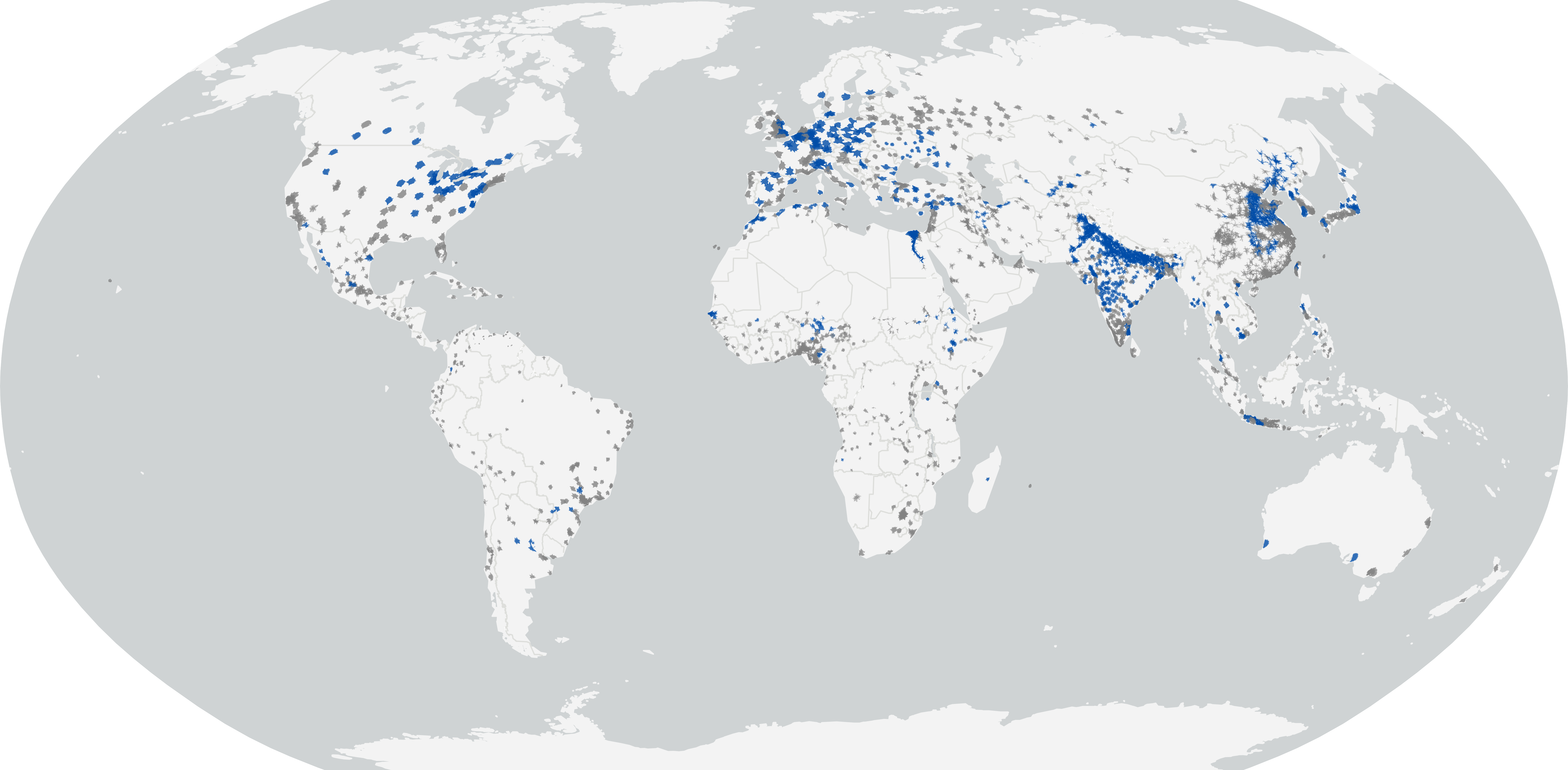
Ultimately, the urban centre selection and generation of the travel-time-based catchments yielded 2,425 unique foodsheds. These had a global extent, with a particularly high density of catchments in Europe, China, India, and parts of Sub-Saharan Africa (Figure 3). My analysis did not account for overlap of these catchments to enforce a maximally inclusive foodshed for each urban centre, though this does not reflect the true distribution of resources in these areas, as more accurately modelled by others (Cattaneo, Nelson, and McMenomy 2021). However, these foodsheds did more accurately represent the true “local” catchment of an urban centre, conforming to each area’s unique terrain, infrastructure, and borders.

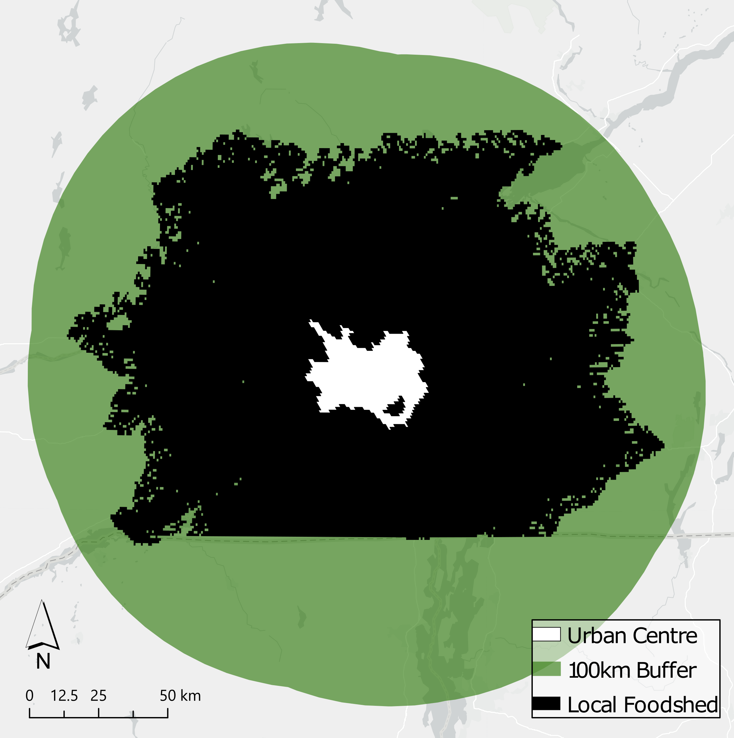
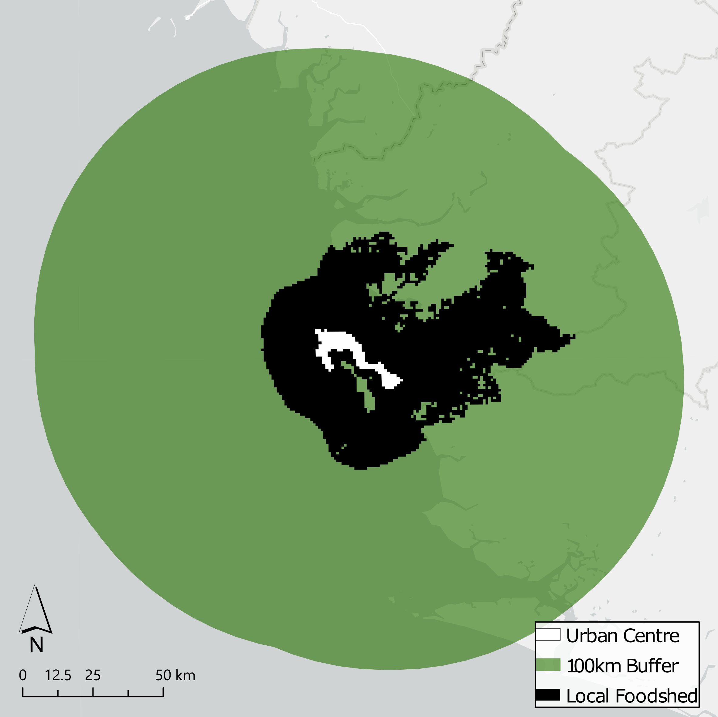
Previous literature addressing local and peri-urban agriculture have primarily used 100 km buffers or the extent of a 30 arc minute cell as a quick way to capture the locality of a given city (Thebo, Drechsel, and Lambin 2014; Kinnunen et al. 2020). Using Weiss et al.’s (2020) Global Motorized Friction Surface’s high resolution (30 arc second, ~1 km at the equator), modern, and global extent, these local and regional catchments represent a more accurate and consistent understanding of the area of influence of a given urban centre. Travel-time-based catchments conform to both the physical and political terrain, adapting to infrastructure conditions, borders, and topography. Its consistency is also an asset: as displayed in Figure 4, while the difference in Montréal’s one-hour catchment and 100 km buffer is subtle, it is far more significant for Freetown.

Foodshed analysis has often been approached in two ways: a globally focused analysis that fully models the complicated interactions and interconnections of global food trade networks, and a locally focused analysis that emphasizes the influence of “local food” in a small food system and offers a critique of globalized food systems (Schreiber et al. 2021; Kinnunen et al. 2020; Nelson et al. 2021). This often leaves researchers with a villainous choice between a low-resolution global investigation or a high-resolution local study that carries fewer significant implications for other areas of the world. This thesis offers a new approach to the study of individual foodsheds at a global scale by generating unique travel-time-based catchments (an analogue for a local foodshed) for each individual urban centre. This individuality, while exceedingly useful, revealed a major limitation to this approach: its calculation time. For my thesis, the generation of the urban centres and their associated catchments took around three full weeks of processing time, not including the time required to learn, write, and debug the code.

Cropland stability

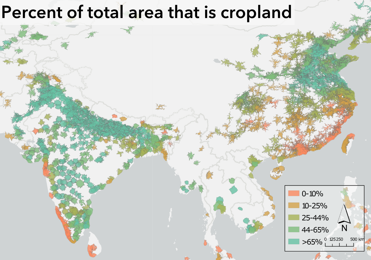
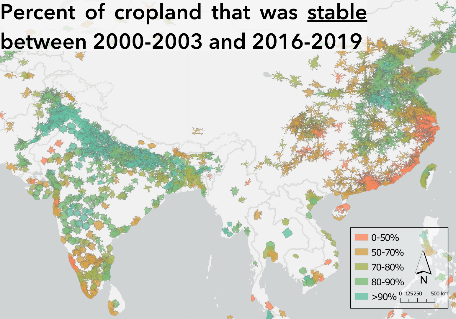
(a) Map of the percent total area that is cropland, with all areas that had \(\ge10\%\) meeting the selection criteria.

Calculating the cropland stability revealed stark geographic patterns in its variation. As displayed in Figure 6 and Table 2, 929 peri-urban foodsheds met both the cropland stability threshold of \(\ge 80\%\) and the total cropland threshold of \(\ge 10\%\). However, their variation mirrors other established cases of large changes in peri-urban land use. Figure 5 demonstrates this, with significant corridors of stable cropland in Northern India and Northern China while the Western coast of India and Southern China both exhibit little total cropland and stable cropland. One of the most interesting scenarios includes areas that met the minimum total cropland requirement but failed to meet the stability criteria, indicating that there is a notable amount of agricultural activity within the peri-urban foodshed that has changed dramatically over 16 years.

(a) The distribution of each foodshed’s percent total cropland with the cutoff of \(\ge10\%\).

Table 2:
A cross-tabulation of each peri-urban foodshed’s total cropland and stable cropland requirements with each combination’s percentage of all 2,425 foodsheds shown.
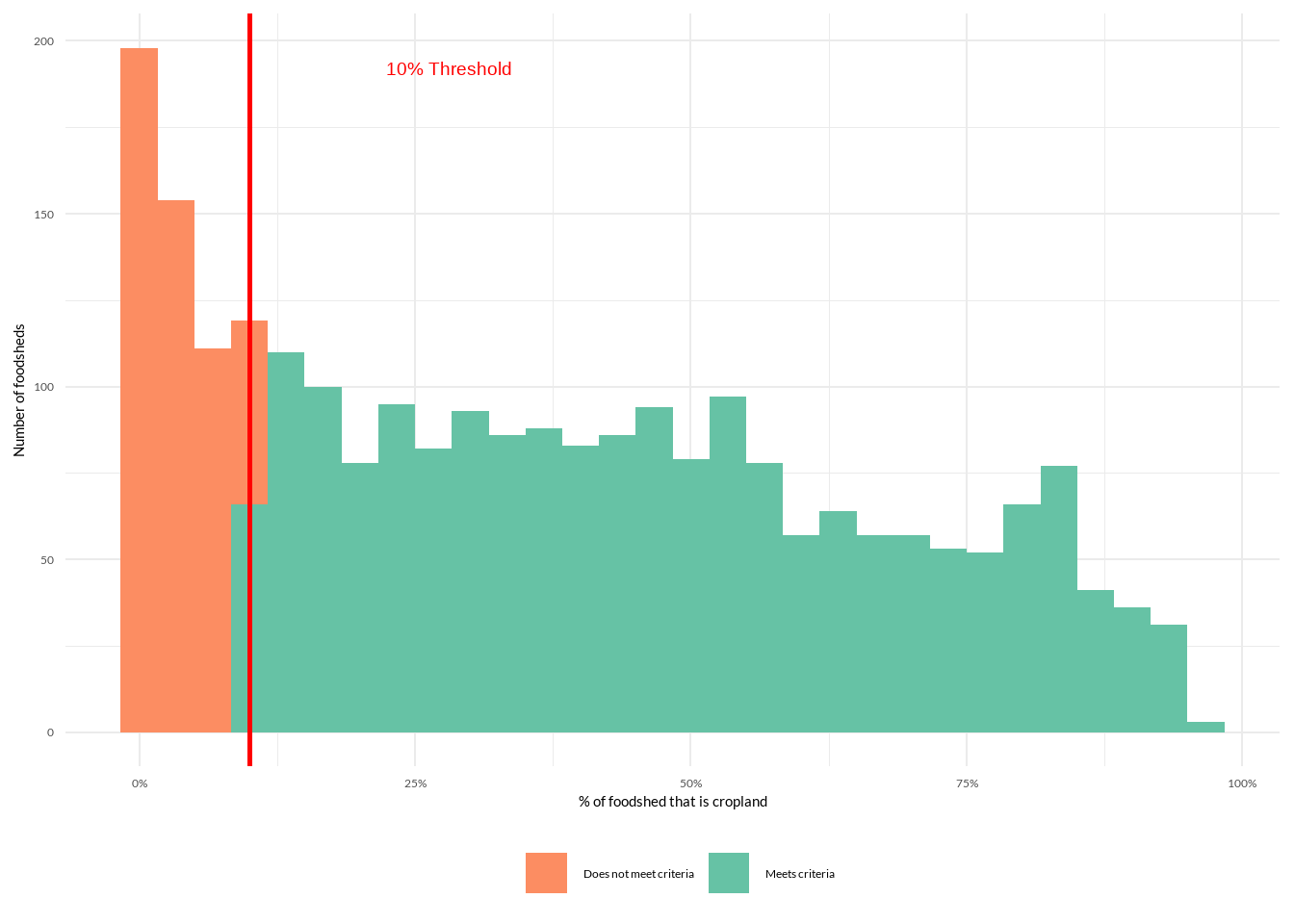
label	variable	Meets stable cropland threshold (>= 80%)
label	variable	FALSE	TRUE
Meets total cropland threshold (>= 10%)	FALSE	491 (20.25%)	25 (1.03%)
Meets total cropland threshold (>= 10%)	TRUE	980 (40.41%)	929 (38.31%)

Evaluating the stability of these croplands accomplishes two tasks: it identifies patterns of rapid peri-urban land use change and offers a powerful tool to validate fixed-time datasets for use with temporally expansive methods. While this approach to evaluating peri-urban cropland stability spans only 16 years of the ideal 30 for an investigation applying climate data, it uses the current best available datasets to do so. The simplicity of this approach allows it to be easily applied for future studies and used within a foodshed to identify areas experiencing major shifts in land use patterns.

A heuristic to determining crop-specific exposure to extreme temperatures

Zooming in on city-specific ‘extreme’ temperatures

I now turn to my proposed method for applying the peri-urban foodshed catchments to assessing climate change applications, specifically, exposure to extreme temperatures. As previously discussed, extreme heat is deadly to crops, but how do we quantify the “extreme”? There are two methods applied in the literature: a threshold temperature above which the crop’s yield begins to fail, or the 95th percentile of maximum temperatures that the crop is exposed to (Jackson et al. 2021; Zhu and Troy 2018; Mueller et al. 2016). The threshold approach involves identifying a crop-specific threshold and identifying growing days with a daily maximum temperature that exceeds that value (Jackson et al. 2021). However, using the same daily maximum temperature data, we can consider the 95th percentile of this data for a given area or cell. This can be helpful to assess the differences in the intensity of exposure to extreme temperatures in different areas, rather than the duration of the exposure. It should be noted that under a normal distribution of temperatures, a higher 95th percentile exposure would also indicate a greater duration of exposures to lower percentiles (e.g., if the 95th percentile value is 41°C and its threshold of 35°C is at the 80th percentile, 20% of all daily maximum temperatures the crop is exposed to will be above its threshold temperature). However, while not requiring a specific threshold temperature, the 95th percentile approach is innately comparative. Previous papers applying this comparative method did so at the regional, national, and continental scales (Mueller et al. 2016; Tuholske et al. 2021).

Proposed framework and workflow

flowchart TD
  a[Peri-urban foodsheds]
  c[(MIRCA2000 Harvested Area)]
  d[(GGCMIP Crop Calendars)]
  c & d --> e(Daily crop-specific mask)
  f[(CHELSA-W5E5 Daily<br/>Maximum Temperature)]
  e & f --> g(Masking temperature data)
  a & g --> h(Selection of foodshed-relevant<br/>temperature data)
  h --> i(Calculation of 95th percentile of daily<br/>maximum temperature observations)

Figure 7: My proposed workflow for determining the crop-specific exposure to extreme heat.

With any city-specific foodshed available for comparison at any selection of scales (and involving any number of possible crops), I selected the 95th percentile application (Figure 7) to avoid the need to determine a crop-specific threshold temperature. This proposed method takes advantage of the three best available products to use with the 1 km foodsheds: irrigation-specific agricultural data from MIRCA2000, recently published global and irrigation-specific crop calendars from GGCMIP, and the 1 km daily temperature data from CHELSA-W5E5 (Portmann, Siebert, and Döll 2010; Jägermeyr, Müller, Minoli, et al. 2021; Karger et al. 2023). While a crop-agnostic approach could be applied (as discussed previously), it is difficult to identify a crop-agnostic growing season. Using GGCMIP’s crop calendars, a number of major crops can be investigated, including spring and winter wheat, maize, rice, and soybeans, as well as more locally relevant crops such as pulses and cassava (Jägermeyr, Müller, Minoli, et al. 2021). In addition to its global extent, it also provides different calendars based on irrigation method, making it ideal for use with MIRCA2000. CHELSA-W5E5, while novel, is being used as a key piece of the high-resolution ISIMIP 3a experiments (Karger et al. 2023). Through a combination of these methods, it is possible to take full advantage of the high resolution of the 1 km peri-urban foodsheds by downscaling both the GGCMI crop calendars and MIRCA2000 to include any 1 km cell that contains a selected crop for an inclusive approach.

In all, this offers a novel approach to determining the specific exposure of peri-urban foodsheds to extreme temperatures and can be adapted to a threshold temperature if preferred. However, I believe this would reduce the power of its conclusions due to the difficulty of establishing a strict threshold for a crop. While this heuristic takes full advantage of the high resolution of the travel-time foodsheds and temperature data, it requires significant computational effort to complete. In its optimized form, every calculation for 1986–2016 will be performed 1.2 trillion times (every tile present in the CHELSA-W5E5 for that time period). Approaching this by breaking the calculations into sectors would be ideal, though cropping such a large dataset does require a lengthy amount of time. Ultimately, it offers foodshed-specific information on individual crops’ exposure to extreme heat, and can be readily extended to extreme cold by using the daily minimum temperatures also provided in CHELSA-W5E5.

Concluding Remarks

In this thesis, I have sought to quantify how croplands have changed in peri-urban regions globally. This is of critical concern, particularly since some of the best, most intensively managed, and most productive croplands are located near cities (Thebo, Drechsel, and Lambin 2014). Though the distance of the travel-time foodsheds vary, less than half of all foodsheds with some cropland had stable agriculture between 2000–2003 and 2016–2019 (Table 2). While it’s difficult to make a direct comparison to Thebo et al.’s (2014) study, my findings from the cropland stability analysis represent a dramatic upheaval of the potential local urban food supplies for many cities. Being urban centre-specific means that this information can be used to identify cities with high cropland stability and those with low cropland stability to compare their policy decisions and other circumstances leading to this result.

Additionally, ensuring that a city’s agriculture is stable is crucial for a temporally expansive analysis. This is especially useful for a temperature focused analysis as it reduces the complexity of attempting to model shifts in peri-urban agriculture for the span of the study. However, with only 38% of peri-urban croplands meeting the stability and cropland requirements (Table 2), this may be less effective as a validation method than I had expected. Nonetheless, determining the extreme temperature exposure is critical to identify which peri-urban food systems are at greatest risk of disruption. Being able to differentiate these peri-urban regions could aid in building more resilient food systems and optimizing the use of climate adaptation technologies to avoid these future disturbances. My proposed framework for calculating these extreme temperature exposures can be the tool to do this, offering city- and crop-specific exposure at a higher resolution to deliver the most relevant extreme temperature information for the world’s population centres.

Works Cited

Becker-Reshef, Inbal, Brian Barker, Alyssa Whitcraft, Patricia Oliva, Kara Mobley, Christina Justice, and Ritvik Sahajpal. 2023. “Crop Type Maps for Operational Global Agricultural Monitoring.” Scientific Data 10 (1): 172. https://doi.org/10.1038/s41597-023-02047-9.

Béné, Christophe, Derek Headey, Lawrence Haddad, and Klaus von Grebmer. 2016. “Is Resilience a Useful Concept in the Context of Food Security and Nutrition Programmes? Some Conceptual and Practical Considerations.” Food Security 8 (1): 123–38. https://doi.org/10.1007/s12571-015-0526-x.

Butler, Ethan E., and Peter Huybers. 2013. “Adaptation of US Maize to Temperature Variations.” Nature Climate Change 3 (1): 68–72. https://doi.org/10.1038/nclimate1585.

Cattaneo, Andrea, Andrew Nelson, and Theresa McMenomy. 2021. “Global Mapping of Urban–Rural Catchment Areas Reveals Unequal Access to Services.” Proceedings of the National Academy of Sciences 118 (2): e2011990118. https://doi.org/10.1073/pnas.2011990118.

Findell, Kirsten L., Alexis Berg, Pierre Gentine, John P. Krasting, Benjamin R. Lintner, Sergey Malyshev, Joseph A. Santanello, and Elena Shevliakova. 2017. “The Impact of Anthropogenic Land Use and Land Cover Change on Regional Climate Extremes.” Nature Communications 8 (1): 989. https://doi.org/10.1038/s41467-017-01038-w.

Florczyk, Aneta, Christina Corbane, Marcello Schiavina, Martino Pesaresi, Luca Maffenini, Michele Melchiorri, Panagiotis Politis, et al. 2019. “GHS-UCDB R2019A - GHS Urban Centre Database 2015, Multitemporal and Multidimensional Attributes,” January. https://doi.org/10.2905/53473144-b88c-44bc-b4a3-4583ed1f547e.

Heino, Matias, Pekka Kinnunen, Weston Anderson, Deepak K. Ray, Michael J. Puma, Olli Varis, Stefan Siebert, and Matti Kummu. 2023. “Increased Probability of Hot and Dry Weather Extremes During the Growing Season Threatens Global Crop Yields.” Scientific Reports 13 (1): 3583. https://doi.org/10.1038/s41598-023-29378-2.

Jackson, Nicole D., Megan Konar, Peter Debaere, and Justin Sheffield. 2021. “Crop-Specific Exposure to Extreme Temperature and Moisture for the Globe for the Last Half Century.” Environmental Research Letters 16 (6): 064006. https://doi.org/10.1088/1748-9326/abf8e0.

Jägermeyr, Jonas, Christoph Müller, Sara Minoli, Deepak Ray, and Stefan Siebert. 2021. “GGCMI Phase 3 Crop Calendar.” https://doi.org/10.5281/ZENODO.5062512.

Jägermeyr, Jonas, Christoph Müller, Alex C. Ruane, Joshua Elliott, Juraj Balkovic, Oscar Castillo, Babacar Faye, et al. 2021. “Climate Impacts on Global Agriculture Emerge Earlier in New Generation of Climate and Crop Models.” Nature Food 2 (11): 873–85. https://doi.org/10.1038/s43016-021-00400-y.

Karg, Hanna, Edmund K. Akoto-Danso, Louis Amprako, Pay Drechsel, George Nyarko, Désiré Jean-Pascal Lompo, Stephen Ndzerem, Seydou Sidibé, Mark Hoschek, and Andreas Buerkert. 2023. “A Spatio-Temporal Dataset on Food Flows for Four West African Cities.” Scientific Data 10 (1): 263. https://doi.org/10.1038/s41597-023-02163-6.

Karger, Dirk Nikolaus, Stefan Lange, Chantal Hari, Christopher P. O. Reyer, Olaf Conrad, Niklaus E. Zimmermann, and Katja Frieler. 2023. “CHELSA-W5E5: Daily 1km Meteorological Forcing Data for Climate Impact Studies.” Earth System Science Data 15 (6): 2445–64. https://doi.org/10.5194/essd-15-2445-2023.

Kinnunen, Pekka, Joseph H. A. Guillaume, Maija Taka, Paolo D’Odorico, Stefan Siebert, Michael J. Puma, Mika Jalava, and Matti Kummu. 2020. “Local Food Crop Production Can Fulfil Demand for Less Than One-Third of the Population.” Nature Food 1 (4): 229–37. https://doi.org/10.1038/s43016-020-0060-7.

Li, Mengmeng, Peter H. Verburg, and Jasper van Vliet. 2022. “Global Trends and Local Variations in Land Take Per Person.” Landscape and Urban Planning 218 (February): 104308. https://doi.org/10.1016/j.landurbplan.2021.104308.

Lobell, David B., Wolfram Schlenker, and Justin Costa-Roberts. 2011. “Climate Trends and Global Crop Production Since 1980.” Science 333 (6042): 616–20. https://doi.org/10.1126/science.1204531.

Monfreda, Chad, Navin Ramankutty, and Jonathan A. Foley. 2008. “Farming the Planet: 2. Geographic Distribution of Crop Areas, Yields, Physiological Types, and Net Primary Production in the Year 2000.” Global Biogeochemical Cycles 22 (1): 2007GB002947. https://doi.org/10.1029/2007GB002947.

Mueller, Nathaniel D., Ethan E. Butler, Karen A. McKinnon, Andrew Rhines, Martin Tingley, N. Michele Holbrook, and Peter Huybers. 2016. “Cooling of US Midwest Summer Temperature Extremes from Cropland Intensification.” Nature Climate Change 6 (3): 317–22. https://doi.org/10.1038/nclimate2825.

Nelson, Andy, Rolf de By, Tom Thomas, Serkan Girgin, Mark Brussel, Valentijn Venus, and Robert Ohuru. 2021. The Resilience of Domestic Transport Networks in the Context of Food Security A Multi-Country Analysis. Background Paper for The State of Food and Agriculture 2021. FAO Agricultural Development Economics Technical Study No. 14. Rome: Food; Agriculture Organization of the United Nations. https://doi.org/10.4060/cb7757en.

Nelson, Andy, Daniel J. Weiss, Jacob van Etten, Andrea Cattaneo, Theresa S. McMenomy, and Jawoo Koo. 2019. “A Suite of Global Accessibility Indicators.” Scientific Data 6 (1): 266. https://doi.org/10.1038/s41597-019-0265-5.

Peters, Christian J., Nelson L. Bills, Jennifer L. Wilkins, and Gary W. Fick. 2009. “Foodshed Analysis and Its Relevance to Sustainability.” Renewable Agriculture and Food Systems 24 (1): 1–7. https://doi.org/10.1017/S1742170508002433.

Portmann, Felix T., Stefan Siebert, and Petra Döll. 2010. “MIRCA2000Global Monthly Irrigated and Rainfed Crop Areas Around the Year 2000: A New High-Resolution Data Set for Agricultural and Hydrological Modeling.” Global Biogeochemical Cycles 24 (1). https://doi.org/10.1029/2008GB003435.

Potapov, Peter, Svetlana Turubanova, Matthew C. Hansen, Alexandra Tyukavina, Viviana Zalles, Ahmad Khan, Xiao-Peng Song, Amy Pickens, Quan Shen, and Jocelyn Cortez. 2022. “Global Maps of Cropland Extent and Change Show Accelerated Cropland Expansion in the Twenty-First Century.” Nature Food 3 (1): 19–28. https://doi.org/10.1038/s43016-021-00429-z.

Ray, Deepak K., James S. Gerber, Graham K. MacDonald, and Paul C. West. 2015. “Climate Variation Explains a Third of Global Crop Yield Variability.” Nature Communications 6 (1): 5989. https://doi.org/10.1038/ncomms6989.

Ray, Deepak K., Paul C. West, Michael Clark, James S. Gerber, Alexander V. Prishchepov, and Snigdhansu Chatterjee. 2019. “Climate Change Has Likely Already Affected Global Food Production.” PLOS ONE 14 (5): e0217148. https://doi.org/10.1371/journal.pone.0217148.

Schiavina, M., S. Freire, A. Carioli, and K. MacManus. 2023. “GHS-POP R2023A - GHS Population Grid Multitemporal (1975-2030).” https://doi.org/10.2905/2FF68A52-5B5B-4A22-8F40-C41DA8332CFE.

Schiavina, M., M. Melchiorri, and M. Pesaresi. 2023. “GHS-SMOD R2023A - GHS Settlement Layers, Application of the Degree of Urbanisation Methodology (Stage i) to GHS-POP R2023A and GHS-BUILT-s R2023A, Multitemporal (1975-2030).” https://doi.org/10.2905/A0DF7A6F-49DE-46EA-9BDE-563437A6E2BA.

Schlenker, Wolfram, and Michael J. Roberts. 2009. “Nonlinear Temperature Effects Indicate Severe Damages to u.s. Crop Yields Under Climate Change.” Proceedings of the National Academy of Sciences 106 (37): 15594–98. https://doi.org/10.1073/pnas.0906865106.

Schreiber, Kerstin, Gordon M. Hickey, Geneviève S. Metson, Brian E. Robinson, and Graham K. MacDonald. 2021. “Quantifying the Foodshed: A Systematic Review of Urban Food Flow and Local Food Self-Sufficiency Research.” Environmental Research Letters 16 (2): 023003. https://doi.org/10.1088/1748-9326/abad59.

Schreiber, Kerstin, Klara J. Winkler, Killian Abellon, and Graham K. MacDonald. 2023. “Planning the Foodshed: Rural and Peri-Urban Factors in Local Food Strategies of Major Cities in Canada and the United States.” Urban Agriculture & Regional Food Systems 8 (1): e20041. https://doi.org/10.1002/uar2.20041.

Seekell, David, Joel Carr, Jampel Dell’Angelo, Paolo D’Odorico, Marianela Fader, Jessica Gephart, Matti Kummu, et al. 2017. “Resilience in the Global Food System.” Environmental Research Letters 12 (2): 025010. https://doi.org/10.1088/1748-9326/aa5730.

Shaw, Brian J., Jasper van Vliet, and Peter H. Verburg. 2020. “The Peri-Urbanization of Europe: A Systematic Review of a Multifaceted Process.” Landscape and Urban Planning 196 (April): 103733. https://doi.org/10.1016/j.landurbplan.2019.103733.

Song, Yanling, Chunyi Wang, Hans W. Linderholm, Yan Fu, Wenyue Cai, Jinxia Xu, Liwei Zhuang, et al. 2022. “The Negative Impact of Increasing Temperatures on Rice Yields in Southern China.” Science of The Total Environment 820 (May): 153262. https://doi.org/10.1016/j.scitotenv.2022.153262.

Song, Yanling, Guangsheng Zhou, Hans W. Linderholm, Junfang Wang, Yong Li, Guofu Wang, Yan Fu, et al. 2023. “Growth of Winter Wheat Adapting to Climate Warming May Face More Low-Temperature Damage.” International Journal of Climatology 43 (4): 1970–79. https://doi.org/10.1002/joc.7956.

Thebo, A. L., P. Drechsel, and E. F. Lambin. 2014. “Global Assessment of Urban and Peri-Urban Agriculture: Irrigated and Rainfed Croplands.” Environmental Research Letters 9 (11): 114002. https://doi.org/10.1088/1748-9326/9/11/114002.

Tuholske, Cascade, Kelly Caylor, Chris Funk, Andrew Verdin, Stuart Sweeney, Kathryn Grace, Pete Peterson, and Tom Evans. 2021. “Global Urban Population Exposure to Extreme Heat.” Proceedings of the National Academy of Sciences 118 (41): e2024792118. https://doi.org/10.1073/pnas.2024792118.

United Nations. 2019. “World Urbanization Prospects: The 2018 Revision (ST/ESA/SER.A/420).” New York: United Nations.

Weiss, D. J., A. Nelson, H. S. Gibson, W. Temperley, S. Peedell, A. Lieber, M. Hancher, et al. 2018. “A Global Map of Travel Time to Cities to Assess Inequalities in Accessibility in 2015.” Nature 553 (7688): 333–36. https://doi.org/10.1038/nature25181.

Weiss, D. J., A. Nelson, C. A. Vargas-Ruiz, K. Gligorić, S. Bavadekar, E. Gabrilovich, A. Bertozzi-Villa, et al. 2020. “Global Maps of Travel Time to Healthcare Facilities.” Nature Medicine 26 (12): 1835–38. https://doi.org/10.1038/s41591-020-1059-1.

Yu, Qiangyi, Liangzhi You, Ulrike Wood-Sichra, Yating Ru, Alison K. B. Joglekar, Steffen Fritz, Wei Xiong, Miao Lu, Wenbin Wu, and Peng Yang. 2020. “A Cultivated Planet in 2010 Part 2: The Global Gridded Agricultural-Production Maps.” Earth System Science Data 12 (4): 3545–72. https://doi.org/10.5194/essd-12-3545-2020.

Zhu, Xiao, and Tara J. Troy. 2018. “Agriculturally Relevant Climate Extremes and Their Trends in the World’s Major Growing Regions.” Earth’s Future 6 (4): 656–72. https://doi.org/10.1002/2017EF000687.

Supplementary Information

Map data source attribution.

Figure 3 projected in Robinson (EPSG:54030). Basemap provided by Esri using data from Esri, TomTom, FAO, NOAA, and the USGS. Peri-urban foodsheds and cropland stability data created by the author.

Figure 4 (a) projected in NAD83 (CSRS) / MTM zone 8 (EPSG:2950). Basemap provided by Esri using data from la Ville de Montréal, Esri Canada, Esri, TomTom, Garmin, FAO, NOAA, USGS, EPA, NPS, NRCan, and Parks Canada.

Figure 4 (b) projected in Sierra Leone 1968 / UTM zone 28N (EPSG:2161). Basemap provided by Esri using data from Esri, OpenStreetMap contributors, TomTom, Garmin, FAO, NOAA, and the USGS.

Figure 5 projected in WGS 1984 (EPSG:4326). Basemap provided by Esri using data from Esri, TomTom, Garmin, FAO, NOAA, and the USGS. Peri-urban foodsheds and cropland stability data created by the author.

Footnotes

In their global analysis of foodsheds, Kinnunen et al. (2020) indicate that pulses, cereals, and rice had the highest rates of potential local fulfillment of their studied crops (22–28%), while tropical roots and maize had much lower local fulfillment potentials (11–16%).↩︎
As I later define, stable cropland is cropland that occurs in the same place in both epochs (i.e. present in 2000–2003 and 2016–2019).↩︎
Though provided in a geographic coordinate system, the GHS-UCDB was generated from projected input data. Florczyk et al. (2019) provides its resolution as “1 km” for this reason.↩︎
While CHELSA-W5E5 Version 1 covers 1979–2016, I selected 1986–2016 as a more relevant 30 year span of climate data due to its greater overlap with the rest of the selected data.↩︎
Otherwise referred to as rook contiguity and queen contiguity, respectively.↩︎

Copyright

2024 Alice H. Clauss